4. Using r3Cseq
4.1 Analyzing the interaction regions for the Myb promoter datasets
3C-seq experiments using the Myb gene promoter as the viewpoint were performed in two cell types from the mouse 12.5 dpc embryo: 1) cells expressing high levels of Myb (fetal liver, FL) and 2) cells expressing low levels of Myb (fetal brain, FB). The latter was used as a negative control in order to appropriately link locus structure to gene expression. We provide two biological replicates for both fetal liver and brain. Since r3Cseq can be used to perform data analysis both with and without replicates, we first demonstrate how to perform data analysis without replicates, followed by data analysis including replicates.
4.1.1 Working without replicates
The following command lines are used to perform r3Cseq analysis for the identification of interaction regions with the Myb promoter.
The first step is to load the r3Cseq package and the example data sets:
> library(r3Cseq)
> library(BSgenome.Mmusculus.UCSC.mm9)
> expFile <-”Myb_prom_FL_rep1.bam”
>contrFile<-”Myb_prom_FB_rep1.bam”
Short reads from the two data sets were mapped to the mouse genome (NCBI37/mm9) using the Bowtie aligner, which provides data output in BAM file format. The two data sets consist of 1) Myb_prom_FL_rep1.bam; the aligned reads of Myb promoter interaction regions in FL erythrocytes, and 2) Myb_prom_FB_rep1.bam; the aligned reads of the FB experiment. We next designated the data from FL erythrocytes as ‘experiment’ and data from FB as ‘control’ with new variables called “expFile” and “contrFile” respectively.
In the next step, an r3Cseq object will be created. The input parameters such as organismName, alignedReadsBamExpFile, alignedReadsBamContrFile, viewpoint_chromosome, viewpoint_primer_forward, viewpoint_primer_reverse, and restrictionEnzyme will be defined. Descriptions of these input parameters can be found in the r3Cseq package documentation.
> my_obj<-new("r3Cseq",organismName='mm9',alignedReadsBamExpFile=expFile,
alignedReadsBamContrFile=contrFile,isControlInvolved=TRUE,viewpoint_chromosome='chr10',
viewpoint_primer_forward='TCTTTGTTTGATGGCATCTGTT',
viewpoint_primer_reverse='AAAGGGGAGGAGAAGGAGGT',
expLabel="Myb_prom_FL_rep1",contrLabel="MYb_prom_FB_rep1",restrictionEnzyme='HindIII')
To load aligned reads from the BAM files, the function getRawReads needs to be executed. The loading process may take a few minutes, depending on the size of the input BAM file, the speed of CPU and the RAM size of the computer that performs the analysis.
>getRawReads(my_obj)
r3Cseq provides two ways to count the number of reads per region; 1) count the number of reads per restriction fragment using the getReadCountPerRestrictionFragment function and 2) count the number of reads per user-defined non-overlapping window size using the getReadCountPerWindow function. The getReadCountPerRestrictionFragment function provides parameters for users to count reads. One method is to count all reads found within the whole restriction fragment (“wholeReads”). Another method is to count only those reads found at the edges of both the 5’end and 3’end of the restriction fragment (“adjacentFragmentEndsReads”). The default parameter is “wholeReads”.
We will now perform the counting analysis per restriction fragment; executing the following command:
>getReadCountPerRestrictionFragment(my_obj)
The 3C-seq protocol always generates a very strong interaction signal at the viewpoint fragment and those immediately adjacent (usually 1 or 2 fragments). This signal is caused by a failure to digest the primary restriction site (resulting in the capture of the neighbouring fragment) and self-ligation of the viewpoint fragment to itself. These signals, although they should always be present, are not informative. Hence, r3Cseq provides the input parameter “nFragmentExcludedReadsNearViewpoint”, which is designed to exclude aligned reads from fragments located up- and downstream of the viewpoint. The default is set to 2, which means we exclude reads located within 2 restriction fragment regions both up- and downstream of the viewpoint from the analysis.
In the next step, r3Cseq uses the calculateRPM function to calculate the reads per million per restriction fragment (RPM) as normalized interaction frequency values.
There are two methods to calculate RPM, which are described in the r3Cseq paper (Thongjuea et al. 2013).
>calculateRPM(my_obj)
After normalization, the getInteractions function will perform statistical analysis to assign statistical values to both cis and trans candidate interaction regions in the datasets from both cell types. A detailed description of the methods for analyzing cis and trans interactions can be found in the r3Cseq paper (Thongjuea et al. 2013).
>getInteractions(my_obj)
To view the results, two functions, expInteractionRegions and contrInteractionRegions, can be used to access the r3Cseq object slot and these functions return a RangedData object that can be easily manipulated by using other basic functions in R.
> expResults<- expInteractionRegions(my_obj)
> expResults
>contrResults<- contrInteractionRegions(my_obj)
>contrResults
r3Cseq provides functions to export raw reads and all interactions to bedGraph file, which is suitable for simple uploading to the UCSC genome browser.
> export3CseqRawReads2bedGraph(my_obj)
> export3Cseq2bedGraph(my_obj)
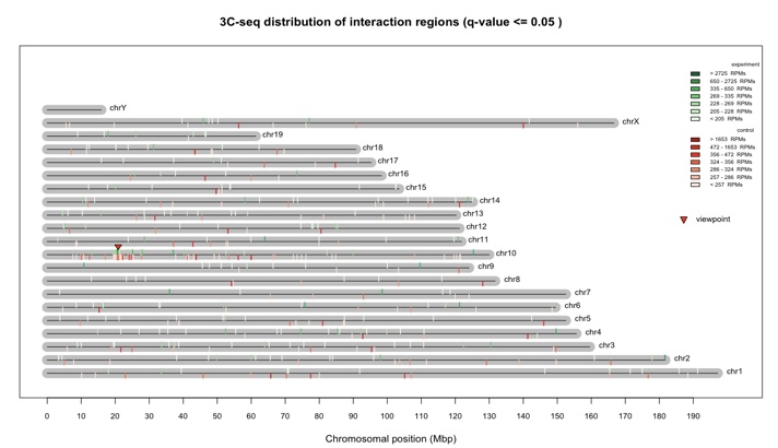
We next used the plotOverviewInteractions function to visualize the overview of interaction regions distributed across the genome.
> plotOverviewInteractions(my_obj)
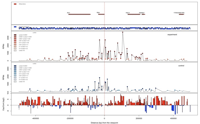
The plotInteractionsNearViewpoint function shows zoomed-in pictures of interaction regions located close to the viewpoint. A user can select the relative distance from the viewpoint (default = 500 kb)
> plotInteractionsNearViewpoint (my_obj)
To plot the interaction regions found on the cis chromosome only (chromosome 10 in this example), the plotInteractionsPerChromosome function can be used.
> plotInteractionsPerChromosome(my_obj,”chr10”)
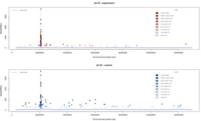
To plot the interaction regions found on individual other chromosomes, the same function as before
can be used.
> plotInteractionsPerChromosome(my_obj,”chr7”)
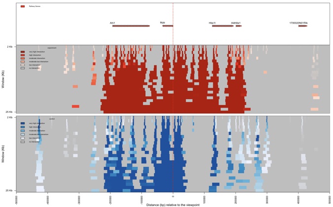
r3Cseq also provides a function to plot domainograms of interaction regions near by the viewpoint. The function plotDomainogramNearViewpoint is designed to visualize the interaction pattern found in cis in both the experiment and control datasets. Users can set the relative distance from the viewpoint (maximum is 500 Kb) and the maximum analysis window (maximum is 50 kb). A user can choose to view the domainogram for the experiment, control or both experiment and control data sets (default=”experiment”). This function is very useful for visualizing differences in the interaction patterns in cis between two conditions. This function may take a few minutes to perform the analysis, depending on the selected distance, maximum window, the speed of CPU and RAM size of the processing computer.
> plotDomainogramNearViewpoint(my_obj)
To create domainograms for both data sets, use the following command:
> plotDomainogramNearViewpoint(my_obj,view=”both”)
Finally, the generate3CseqReport function can be used to generate a summary report containing
the r3Cseq analysis results. This report contains a PDF file with all plots and a text file with the
interaction regions.
> generate3CseqReport(my_obj)
To promptly switch data analysis from a fragment based to a window based setting, users DO NOT
have to re-initialize the r3Cseq class. They can just use the existing class and redo the analysis
steps starting from calculating the number of reads using the getReadCountPerWindow function instead.
4.1.2 working with replicates
From the example data sets section, we can download two replicates of the Myb promoter viewpoint 3C-seq fetal liver experiment (Myb_prom_FL_rep1.bam and Myb_prom_FL_rep2.bam, the aligned reads of Myb promoter interaction regions in FL erythrocytes), and two replicates of the same experiment in fetal brain cells (Myb_prom_FB_rep1.bam and Myb_prom_FB_rep2.bam). We next assigned the datasets from FL erythrocytes as ‘experiment’ and datasets from FB as ‘control’. r3Cseq provides replicate analysis by building a r3CseqInBatch class. First the r3CseqInBatch class needs to be initialized and provided with the input parameters. Descriptions of these input parameters can be found in the r3Cseq package documentation.
*change the path of the bamFileDirectory for your data analysis
> library(r3Cseq)
> myBatch_obj<-new("r3CseqInBatch",organismName='mm9',restrictionEnzyme='HindIII',isControlInvolved=TRUE,bamFilesDirectory="/home/supat/3C_Seq_replicates/bam",viewpoint_chromosome='chr10',viewpoint_primer_forward='TCTTTGTTTGATGGCATCTGTT',viewpoint_primer_reverse='AAAGGGGAGGAGAAGGAGGT',BamExpFiles=c("Myb_prom_FL_rep1.bam","Myb_prom_FL_rep2.bam"),
BamContrFiles=c("Myb_prom_FB_rep1.bam","Myb_prom_FB_rep2.bam"),
expBatchLabel=c("Myb_FL1","Myb_FL2"),contrBatchLabel=c("Myb_FB1","Myb_FB2"))
To load aligned reads from the multiple BAM files, the getBatchRawReads function has to be executed. The loading process may take a few minutes, depending on the size of the input BAM files, the speed of the CPU and the RAM size of the computer that performs the analysis.
>getBatchRawReads(myBatch_obj)
r3Cseq provides two read counting functions, similar to those used when working without replicates:
1) counting the number of reads per restriction fragment, using the getBatchReadCountPerRestrictionFragment function and 2) counting the number of reads per non-overlapping window size, using the getBatchReadCountPerWindow function.
In this example we perform the read counting analysis with a 20 kb window by executing the following command:
>getBatchReadCountPerWindow(myBatch_obj, windowSize=20e3)
We next used the calculateBatchRPM function to calculate the reads per million per restriction fragment size (RPM) as normalized interaction frequency values.
>calculateBatchRPM(myBatch_obj)
After normalization, the getBatchInteractions function can be used to assign p and q-values (both for in cis and trans interactions) to identify candidate interaction regions in both datasets. r3Cseq further provides two
ways of determine significant interactions among the biological replicates: 1) all identified interactions from
the individual replicates are combined using the “union” parameter as input method and 2) only the
identified interactions presented in all individual replicates are combined using the “intersection”
parameter as input method. The default parameter is “union”. The getBatchInteractions function will also determine the identified interactions per individual replicate and saves them into a text file during the
running process.
>getBatchInteractions(myBatch_obj)
To only obtain those interactions presented in all individual replicates, the following commands can be used:
>getBatchInteractions(myBatch_obj,method=”intersection”)
The exportBatchInteractions2text function can be used next to export all of the identified interactions to text file format.
> exportBatchInteractions2text(myBatch_obj)
For visualization of the identified interactions among replicates, similar functions can be utilized as those used when working without replicates:
> plotOverviewInteractions(myBatch_obj)
> plotInteractionsNearViewpoint (myBatch_obj)
> plotInteractionsPerChromosome(myBatch_obj,”chr10”)
5. How to cite r3Cseq?
If you find this resource useful, please cite our paper:
Supat Thongjuea, Ralph Stadhouders, Frank Grosveld, Eric Soler and Boris Lenhard: r3Cseq:
an R/Bioconductor package for the discovery of long-range genomic interactions from chromosome
conformation capture and next-generation sequencing data. Nucleic acids research, 41, e132.